
At Edgemesh our backend is responsible for capturing and querying across millions of real user metrics and browser cache states every day. On any typical day, Edgemesh records:
- 2-40 million Level 1 RUM stats (Pageviews)
- 10-100 million Cache states (Browser cache integrity and registration)
- 500 million - 4 billion Level 2 RUM stats (Waterfall)
Typically, companies will implement pipelines using a set of logical components to deal with the ingestion, analysis and storage or data streams like ours. Examples include:
- Data Capture / ETL / Stream Processing : Custom Code , StreamBase , Dataflow
- Messaging: Kafka , NSQ or managed solutions such as GCP Pub/Sub
- Database : Clickhouse, InfluxDB or managed “Big Data’ solutions like BigQuery or RedShift
- Analytics / OLAP / Warehouse: Apache Arrow , SnowFlake
- AI / Advanced Modeling: Tensorflow etc
These result in ‘scalable’ architectures that are … complicated. There are multiple vendor specific languages and systems - each with their own operational complexity. Below is an example of a ‘modern’ pipeline.
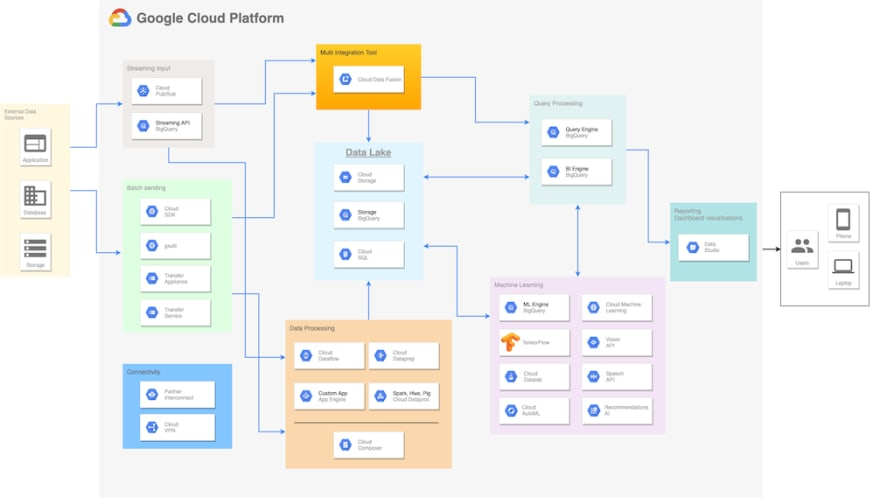
Instead of this multi-headed hydra - at Edgemesh we use a single 129kB binary for all these functions, called Elle. All running on a single machine (with failover).
An Ode to K
Elle is modeled after Kdb+ , the insanely fast time series database employed at nearly every bank and exchange on Wall Street (where I used it for ~15 years). Kdb+ is a column-oriented, vector database with a built in message bus and powerful array language (Q). Kdb was developed by Arthur Whitney, the renowned computer scientist and designer of the array languages A+, K , Q and now K9 (Shakti). Although Kdb+ allows for standard SQL queries - the real power is the Q language itself. Elle is our implementation of a Kdb like system with (nearly) full support for executing Q code.
My first experience with array languages was K (Kdb) - the predecessor to Q (Kdb+) at Appian around 2000. Unfortunately, the K from this era was lost to time - but a former intern of mine, Kevin Lawler , has implemented a fantastic recreation called Kona. Other implementations of later versions of K dialects exist as well (and some very fast).
As a C programmer, K was a ‘mind shattering’ introduction to the power of keeping data and code side by side. Most importantly, the power of ‘array programming’ showed how one could develop entire data systems without loops and massively simpler code. As an example, here is how one might increment values in an array in C:
{% code-block language="c" %}
#include <stdio.h>
int main() {
int A[4] = {1,2,3,4};
int n = sizeof(A)/sizeof(int);
for (int i=0; i < n; i++){
A[i]+=1;
printf("%d ",A[i]);
};
}
{% code-block-end %}
But in array languages, we can simply operate on the array directly. For example
{% code-block language="q" %}
l>a:1 2 3 4
1 2 3 4
l>a+1
2 3 4 5
{% code-block-end %}
We can also interact with indices as vectors. For example, let’s set the values at index 0 and 2 to 10. The set operator (:) is akin to the = operator in C.
{% code-block language="q" %}
l>a[0 2]:10
l>a
10 2 10 4
{% code-block-end %}
A Database is just a Dictionary
If we think of a table in a column oriented fashion, we can see that tables are really just a set of arrays. Let’s take a look at this a bit more in depth:
{% code-block language="q" %}
//Let’s make 3 arrays, a b and c
l>a: 1 2 3 4
l>b: 10 20 30 40
l>c: 100 200 300 400
l>a
1 2 3 4
l>b
10 20 30 40
l>c
100 200 300 400
{% code-block-end %}
Now let’s create a dictionary - which is similar to a map. The format here is keys!values.
{% code-block language="q" %}
l>d:`a`b`c!(a;b;c)
l>d
a| 1 2 3 4
b| 10 20 30 40
c| 100 200 300 400
// we can now index into this dictionary with a key
// similar to the index in an array
l>d[`a]
1 2 3 4
l>d[`b]
10 20 30 40
// A table is just a transposed (flipped) dictionary.
// Think of turning a map on its side
l>t:flip d
l>t
a b c
--------
1 10 100
2 20 200
3 30 300
4 40 400
// and tables can have SQL executed over them
l>select sum a from t
a
-
6
// tables have indices , but without a key they act like arrays
l>t[0 2]
a b c
--------
1 10 100
3 30 300
// if we “key” a table, we can then use that as our index:
l>t:`a xkey t
l>t
a| b c
-| ------
1| 10 100
2| 20 200
3| 30 300
l>t[2]
b| 20
c| 200
{% code-block-end %}
Putting Array Programming to Work - Making Histograms
At Edgemesh we want to keep the richness of real user metrics datasets without storing everything. Keeping an average of performance metrics, is easy - but it's meaningless. Instead, we are going to keep histograms and some high level summary stats.
Let's say we want to keep a count of items in 1 second buckets. Our buckets would look like:
{% code-block language="q" %}
start end cnt
-------------
0 1 4
1 2 9
2 3 2
3 4 7
4 5 0
5 6 1
6 7 9
7 8 2
8 9 1
9 Inf 8
{% code-block-end %}
The first bucket (row) is a count of items that had a timing between 0 - 1 seconds, the next bucket is a count of items that had a timing between 1 - 2 seconds etc.
If we know what the bucket sizes are, and they are uniform (here they are uniform 1 second increments) - then a histogram is simply the array of the counts.
{% code-block language="q" %}
4 9 2 7 0 1 9 2 1 8
{% code-block-end %}
But what if we want to get the median value from a histogram? Or the 95th percentile? Well ... array programming for the win!
{% code-block language="q" %}
// Remember - Q code reads right to left
// So we start on the right with sum[array] = 43,
// Then we get our running sum (sums[array]) inside the ()
// and finally divide the running sum array by 43
l>(sums 4 9 2 7 0 1 9 2 1 8)%sum 4 9 2 7 0 1 9 2 1 8
// the running sum divided by the total is the density per bucket
0.093 0.302 0.349 0.512 0.512 0.535 0.744 0.791 0.814 1
// let's set variable a to the result
l>a:(sums 4 9 2 7 0 1 9 2 1 8)%sum 4 9 2 7 0 1 9 2 1 8
// Now finding the median is the last index
// where the density is NOT more than .5
// Let’s break this down
// We can get a boolean array
// where true (1b) represents when the value is <.5
l>a<.5
1110000000b
// we can use the where operator
// to find the indices where the boolean array is true
l>where a<.5
0 1 2
// and the median is just the last index so
l>last where a<.5
2
// index 2 means the median here is between 2-3 seconds
// If the array was large, we might want to take advantage
// of the fact that it’s always sorted in ascending order.
// So we can use binary search which is the bin operator.
// X bin y means
// find the last index in X that is strictly not greater than y
l>a bin .5
2
// index 2 means the median here is between 2-3 seconds
// array languages like APL/K/Q make calculating percentiles like this trivial
l>`p25`p50`p75`p90`p95`p99!((sums 4 9 2 7 0 1 9 2 1 8)%sum 4 9 2 7 0 1 9 2 1 8 )bin .25 .5 .75 .9 .95 .99
p25| 0
p50| 2
p75| 6
p90| 8
p95| 8
p99| 8
{% code-block-end %}
In the next article we will see how this 1 line function allows us to calculate histograms on streaming inputs at ~8 millions records per second per core.


