
See Part 1 of this series for a brief overview of array programming in Q
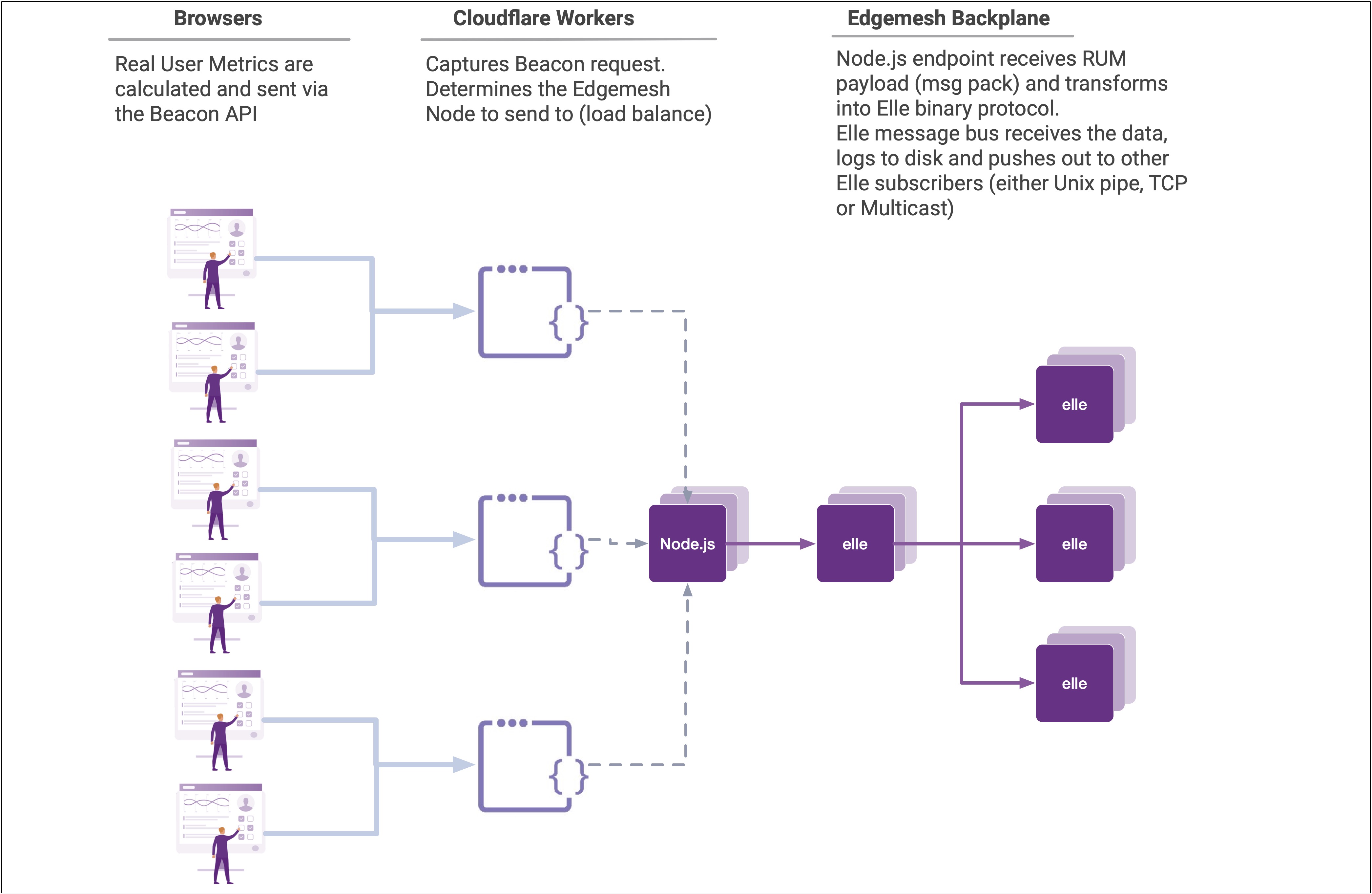
Every time a new customer signs up for Edgemesh, our Real User Metrics feature is enabled on their visitors browser. This helps the Edgemesh Service Worker and backend determine which assets are the best candidates for automatic prefetching as well as providing deep introspection into the real customer experience from a performance standpoint.
It also means that we capture, analyze and store a whole bunch of data.
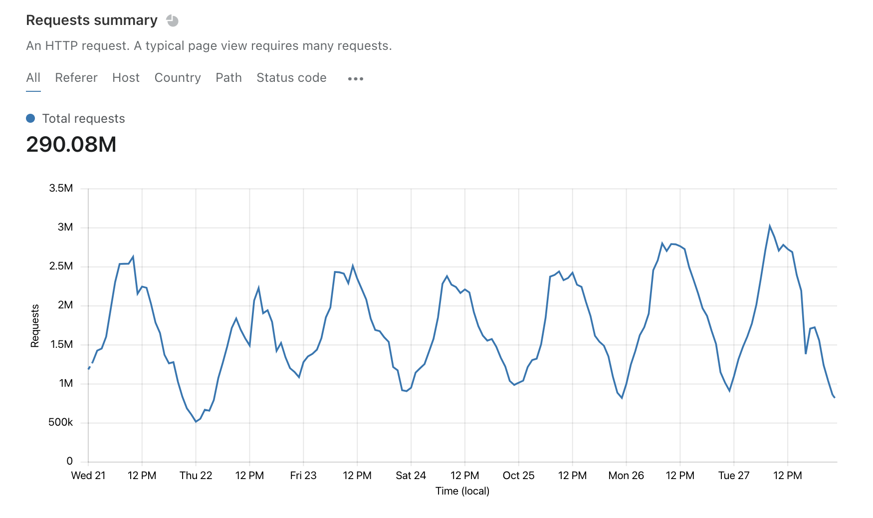
During peak holiday traffic, Edgemesh might capture, parse, analyze and store as much as 80 million Level 1 (Page Level) and 4 billion Level 2 (Resource Level) stats in a 24 hour period. With Edgemesh version 4 we've also added new metrics such as Long Task Events, error events and nested structures such as the Server Timing API.
To ensure that we can keep up with the inevitable 'hug of death' - we need to make sure every CPU cycle in our data pipeline is as efficient as possible. And this is where array programming comes to the rescue!
Keeping value: a.k.a averages are for children
What we want to do is keep the richness of the datasets without storing everything. Keeping an average of performance metrics is easy - but it's also useless. Instead, we are going to keep histograms and some high level summary stats.
To start, let's have a look at the simplest data set - the Level 1 Navigation statistics. These are the traditional metrics one looks at when referring to 'Page Load Time' - although... it's not just one metrics.
Pre-connection Timing
There is really just one metric here, the unload time. This is a commonly overlooked metric as it is actually the time it takes to finish unloading a page before loading a new one. As an example, if you have a page with a bunch of data that needs to be submitted and isn't using the Beacon API or better yet an orthogonal Service Worker - the browser has to finish sending the data for the last page before it can service the navigation request for the nest page. We have seen this hundreds of times, often with a client side performance tool reporting real user metrics stats!
{% code-block language="q" %}
unloadTime: `int$(); // the time until the unload event completes
{% code-block-end %}
Server (backend) Timing:
This is the more familiar set of metrics that define how long the server takes to respond with the initial data.
{% code-block language="q" %}
sslTime: `int$(); // the time taken by the SSL negotiation
tcpTime: `int$(); // the time to establish the TCP connection
dnsTime: `int$(); // the dns lookup time
reqTime: `int$(); // the request time
resTime: `int$(); // the response time
ttfb: `int$(); // the time to first byte
{% code-block-end %}
Client (frontend) Timing
This is the set of metrics that define actual user experience markers. For example, the Paint Timing API allows you to calculate things like how long a browser took to go from blank to non-blank (First Paint) or the new Web Vitals favorite - Largest Contentful Paint.
{% code-block language="q" %}
workerTime: `int$(); // the service worker time to fetch an asset from Origin
fetchTime: `int$(); // the time to fetch assets (including caches)
startRender: `int$(); // the time until rendering begins
firstContentfulPaint: `int$(); // the time to first paint
largestContentfulPaint: `int$(); // the largest contentful paint
contentLoaded: `int$(); // the time until the contentLoaded event
onload: `int$(); // the onload time for the page (window.onload)
pageLoad: `int$(); // the pageload time
firstCPUIdle: `int$(); // time until CPU was idle
{% code-block-end %}
Page Telemetry
This is additional information about engagement with the page, the page size, the number of assets required as well Edgemesh specific information such as the number of assets that were served from the Edgemesh managed cache.
{% code-block language="q" %}
firstClick: `int$(); // the time until a click event was received
firstKeypress: `int$(); // the time until a keypress event was received
firstScroll: `int$(); // the time until a scroll event was received
firstMousemove: `int$(); // the time until a scroll event was received
inputDelay: `int$(); // the first input delay
timeOnPage: `int$(); // the time on page in Ms
assetCnt: `int$(); // the count of the assets
accelAssetCnt `int$(); // the count of the accelerated (cached) assets
transferSize: `int$(); // size in bytes for the page send (including header)
encodedSize: `int$(); // the (possibly) compressed size
decodedSize: `int$(); // the decompressed size in bytes
{% code-block-end %}
Let's have a look at some sample data inputs, saved here in a table called 'sample'.
{% code-block language="q" %}
l>sample
time unloadTime sslTime tcpTime dnsTime reqTime resTime ttfb fetchTim..
-----------------------------------------------------------------------------..
00:09:18.739 891 739 371 751 741 507 358 921 ..
00:23:21.098 680 21 467 340 756 348 956 655 ..
00:45:29.097 544 457 687 690 626 164 261 791 ..
00:52:09.577 633 955 661 617 493 440 313 22 ..
...
{% code-block-end %}
Choosing bin sizes and bounds
For most performance based metrics, there is some level of granularity which just isn't necessary. For example, do you really need millisecond precision on Time To First Byte, or is 10 millisecond precision enough? In addition - nearly all web performance metrics have an inherent jitter in the metrics themselves - probably on the order of 10s of milliseconds. As such, if we can keep our metrics in say 50ms buckets we will cover most of the details.
Now that we know most (but not all) metrics will be in 50ms increments - it's a question of length. A histogram is really just a vector or some length. As a habit, I always like to work in powers of 2 if possible - but as a close second multiples of 64. Since Elle has SIMD compression on integer vectors, it would be nice to have the length be either 128 or 256 in 32 bit Integers.
Unfortunately, at 128 buckets with 50ms precision our last bucket would hold the count of all samples that took more than 6.4 seconds (50ms * 128). Although I deeply wish that all sites recorded metrics below this threshold - in reality we need to go up one level. In the chart below we can see that 92.9% of samples of the Time To Interactive are less than 6.4s... but that leaves almost 7% of samples pinned to the last bucket - which is too big.
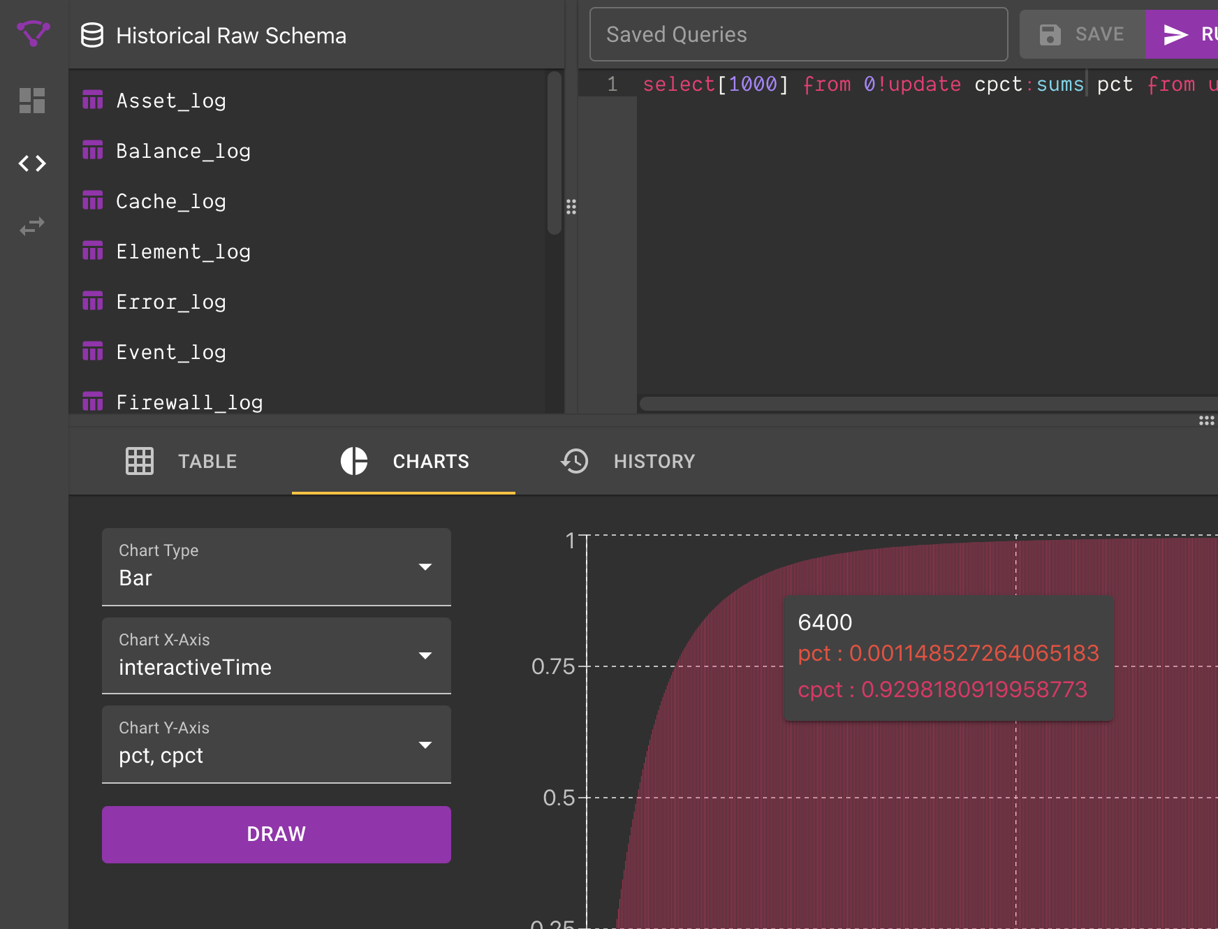
As a general rule of thumb, you want to ensure that your last bin has <=1% of all known samples. At 256 entries we can be more comfortable our outliers are accurately reflected in our histogram while having a granularity that is small enough to be useful. Better to be safe now than to be sorry later!
After a bit of quick data checking with real world metrics - we can hone in on the precision bounds for histograms of length 256 for each metric:
{% code-block language="q" %}
metric | precisionMs maxValue
----------------------| --------------------
unloadTime | 10 2560
sslTime | 10 2560
tcpTime | 10 2560
dnsTime | 10 2560
reqTime | 10 2560
resTime | 10 2560
ttfb | 25 6400
fetchTime | 25 6400
workerTime | 25 6400
startRender | 50 12800
firstContentfulPaint | 50 12800
interactiveTime | 50 12800
largestContentfulPaint| 50 12800
contentLoaded | 50 12800
onload | 50 12800
pageLoad | 50 12800
firstCPUIdle | 50 12800
{% code-block-end %}
Efficient and accurate histogram calculation and storage
As stated before, a histogram is simply a count of items in a bucket (bin). If we know the bin size ahead of time, we can simply store the counts. Elle, like other APL/K/Q descendants, allows for storage and query over nested vectors so we can feel free to store our histogram arrays in a column.
Let's start the calculation. We start by allocating an empty array of 256 zeros.
Here we are saying "take (#) 256 items of the number 0"
{% code-block language="q" %}
l>256#0
0 0 0 0 0 0 0 0 0 0 0 0 0 0 0 0 0 0 0 0 0 0 0 0 0 0 0 0 0 0 0 0 0 0 0 0 0 0 0..
{% code-block-end %}
Now when we get a metric value (say firstContentfulPaint), we look at our bin precision (50ms) and we can simply : divide the input by precision then floor it to get the 'index' we bump in our histogram array,
{% code-block language="q" %}
//sample input value is, 535
l> 535%50
10.7
// now we can floor it - this is helpful since floor is an AVX accelerated operation here
l> floor 535%50
10
//so in our blank array (called blankBuffer here), we need to update index 10 to be +1 sample
l>blankBuffer:256#0
l>blankBuffer
0 0 0 0 0 0 0 0 0 0 0 0 0 0 0 0 0 0 0 0 0 0 0 0 0 0 0 0 0 0 0 0 0 0 0 0 0 0 0..
// let's see the current value of index 10
l>blankBuffer[10]
0
// the obvious solution is the cleanest - just set the index (10) equal to +1 (+:1)
l>blankBuffer[10]+:1;
// another form of this is using the @[list;index;function;arg] construction
// this is a handy form because +:1 assumes that there is a variable we are 'resetting'
// if we wanted to keep a version of this without a variable we can just do
l>@[256#0;10;+;1]
0 0 0 0 0 0 0 0 0 0 1 0 0 0 0 0 0 0 0 0 0 0 0 0 0 0 0 0 0 0 0 0 0 0 0 0 0 0 0..
{% code-block-end %}
This all seems very straight forward... but the power of array languages are... well... arrays.
{% code-block language="q" %}
l>blankBuffer[1 3 5 7]+:1; // increment multiple indices of blankBuffer at once
l>blankBuffer
0 1 0 1 0 1 0 1 0 0 0 0 0 0 0 0 0 0 0 0 0 0 0 0 0 0 0 0 0 0 0 0 0 0 0 0 0 0 0..
{% code-block-end %}
Making it work with real data
Since we will always have 256 buckets per metric, all we need to have defined is the bin size (precision). We can keep these in a dictionary (map) to make our life easier.
{% code-block language="q" %}
l>metricBZ
unloadTime | 10
sslTime | 10
tcpTime | 10
dnsTime | 10
reqTime | 10
resTime | 10
ttfb | 25
fetchTime | 25
workerTime | 25
startRender | 50
firstContentfulPaint | 50
interactiveTime | 50
largestContentfulPaint| 50
contentLoaded | 50
onload | 50
pageLoad | 50
firstCPUIdle | 50
{% code-block-end %}
We now have everything we need to compress a table of Level 1 Navigation metrics into a set of histograms per metric.
{% code-block language="q" %}
//let's have a look at our sample table ... which is 1 million records long
l>sample
time unloadTime sslTime tcpTime dnsTime reqTime resTime ttfb fetchTim..
-----------------------------------------------------------------------------..
00:09:18.739 891 739 371 751 741 507 358 921 ..
00:23:21.098 680 21 467 340 756 348 956 655 ..
00:45:29.097 544 457 687 690 626 164 261 791 ..
00:52:09.577 633 955 661 617 493 440 313 22 ..
00:53:12.907 208 719 416 454 983 607 497 173 ..
01:01:20.864 383 169 452 396 697 207 545 54 ..
01:07:32.507 733 51 234 892 588 87 724 954 ..
... +999993
// getting the keys of our metricBSZ dictionary returns a list of columns that hold
// performance metrics
l>key metricBSZ
`unloadTime`sslTime`tcpTime`dnsTime`reqTime`resTime`ttfb`fetchTime`workerTime..
// tables can be indexed by columns ... and return the column values :)
// with each row being the column of the sample table (transposed)
l>sample[key metricBSZ]
891 680 544 633 208 383 733 234 ..
739 21 457 955 719 169 51 852 ..
371 467 687 661 416 452 234 3 ..
751 340 690 617 454 396 892 276 ..
741 756 626 493 983 697 588 981 ..
507 348 164 440 607 207 87 35 ..
358 956 261 313 497 545 724 444 ..
921 655 791 22 173 54 954 294 ..
468 464 778 290 355 796 983 805 ..
139 862 894 251 928 548 381 65 ..
154 610 676 870 505 166 700 794 ..
912 910 357 487 427 101 211 652 ..
181 13 525 195 185 294 68 610 ..
228 733 486 473 694 189 720 388 ..
607 358 467 341 995 248 3 436 ..
21 706 675 749 740 473 593 788 ..
698 345 920 390 689 398 337 392 ..
// since we know we indexed into the table, we can divide by our metricBSZ dictionary
// which has the handy feature of giving back the column headers (the key from the
// dictionary promotes)
l>sample[key metricBSZ]%metricBSZ
unloadTime | 89.1 68 54.4 63.3 20.8 38.3 ..
sslTime | 73.9 2.1 45.7 95.5 71.9 16.9 ..
tcpTime | 37.1 46.7 68.7 66.1 41.6 45.2 ..
dnsTime | 75.1 34 69 61.7 45.4 39.6 ..
reqTime | 74.1 75.6 62.6 49.3 98.3 69.7 ..
resTime | 50.7 34.8 16.4 44 60.7 20.7 ..
ttfb | 14.32 38.24 10.44 12.52 19.88 21.8 ..
fetchTime | 36.84 26.2 31.64 0.88 6.92 2.16 ..
workerTime | 18.72 18.56 31.12 11.6 14.2 31.84 ..
startRender | 2.78 17.24 17.88 5.02 18.56 10.96 ..
firstContentfulPaint | 3.08 12.2 13.52 17.4 10.1 3.32 ..
interactiveTime | 18.24 18.2 7.14 9.74 8.54 2.02 ..
largestContentfulPaint| 3.62 0.26 10.5 3.9 3.7 5.88 ..
contentLoaded | 4.56 14.66 9.72 9.46 13.88 3.78 ..
onload | 12.14 7.16 9.34 6.82 19.9 4.96 ..
pageLoad | 0.42 14.12 13.5 14.98 14.8 9.46 ..
firstCPUIdle | 13.96 6.9 18.4 7.8 13.78 7.96 ..
// and we can floor a full dictionary (floor across each row)
l>floor sample[key metricBSZ]%metricBSZ
unloadTime | 89 68 54 63 20 38 73 23 37 21 56 68 52 97 38 ..
sslTime | 73 2 45 95 71 16 5 85 26 65 72 10 42 83 34 ..
tcpTime | 37 46 68 66 41 45 23 0 38 51 86 6 70 31 43 ..
dnsTime | 75 34 69 61 45 39 89 27 42 30 54 29 38 79 95 ..
reqTime | 74 75 62 49 98 69 58 98 18 62 75 42 40 44 2 ..
resTime | 50 34 16 44 60 20 8 3 5 27 34 72 5 96 80 ..
ttfb | 14 38 10 12 19 21 28 17 11 7 20 20 4 35 9 ..
fetchTime | 36 26 31 0 6 2 38 11 14 31 8 32 2 12 23 ..
workerTime | 18 18 31 11 14 31 39 32 31 15 7 8 1 25 32 ..
startRender | 2 17 17 5 18 10 7 1 4 12 18 13 7 9 3 ..
firstContentfulPaint | 3 12 13 17 10 3 14 15 0 4 8 5 1 10 0 ..
interactiveTime | 18 18 7 9 8 2 4 13 8 0 18 0 14 10 3 ..
largestContentfulPaint| 3 0 10 3 3 5 1 12 10 5 16 5 2 13 17 ..
contentLoaded | 4 14 9 9 13 3 14 7 15 11 11 10 9 12 17 ..
onload | 12 7 9 6 19 4 0 8 18 17 2 3 13 7 3 ..
pageLoad | 0 14 13 14 14 9 11 15 6 4 19 5 11 17 4 ..
firstCPUIdle | 13 6 18 7 13 7 6 7 0 18 4 1 18 9 3 ..
// this is our index into our blank buffers ... but we need to make sure the max value
// is the max available index (255). So let's cap these using the min (&) operator
l>255&floor sample[key metricBSZ]%metricBSZ
unloadTime | 89 68 54 63 20 38 73 23 37 21 56 68 52 97 38 ..
sslTime | 73 2 45 95 71 16 5 85 26 65 72 10 42 83 34 ..
tcpTime | 37 46 68 66 41 45 23 0 38 51 86 6 70 31 43 ..
dnsTime | 75 34 69 61 45 39 89 27 42 30 54 29 38 79 95 ..
reqTime | 74 75 62 49 98 69 58 98 18 62 75 42 40 44 2 ..
resTime | 50 34 16 44 60 20 8 3 5 27 34 72 5 96 80 ..
ttfb | 14 38 10 12 19 21 28 17 11 7 20 20 4 35 9 ..
fetchTime | 36 26 31 0 6 2 38 11 14 31 8 32 2 12 23 ..
workerTime | 18 18 31 11 14 31 39 32 31 15 7 8 1 25 32 ..
startRender | 2 17 17 5 18 10 7 1 4 12 18 13 7 9 3 ..
firstContentfulPaint | 3 12 13 17 10 3 14 15 0 4 8 5 1 10 0 ..
interactiveTime | 18 18 7 9 8 2 4 13 8 0 18 0 14 10 3 ..
largestContentfulPaint| 3 0 10 3 3 5 1 12 10 5 16 5 2 13 17 ..
contentLoaded | 4 14 9 9 13 3 14 7 15 11 11 10 9 12 17 ..
onload | 12 7 9 6 19 4 0 8 18 17 2 3 13 7 3 ..
pageLoad | 0 14 13 14 14 9 11 15 6 4 19 5 11 17 4 ..
firstCPUIdle | 13 6 18 7 13 7 6 7 0 18 4 1 18 9 3 ..
layoutShift | 172 11 112 187 47 238 27 42 19 243 239 135 12 128 34 ..
// now to compress each row into a histogram ... let's make a function {}
// this one is unnamed (lambda). We are going to use our amend @[] form as before
// except we also want to make sure any indexes <0 are removed
// This is due to some metrics calculating wrong (e.g. ttfb of -100ms)
// Every function has 3 implicit arguments (x,y and z) ... just like math
// here's our function:
// we amend (@) into the list 256#0 at the index from x where the input (x) is >=0, and we add (+) 1
{@[256#0;x where x>=0;+;1]}
// now we want to run this against each row from above (x in above is a row of data)
l>{@[256#0;x where x>=0;+;1]}each 255&floor sample[key metricBSZ]%metricBSZ
unloadTime | 2 2 0 1 1 1 0 0 1 0 1 0 2 0 1 0 1 1 1 0 1 4 1 2 0 ..
sslTime | 0 0 1 0 0 2 1 2 3 1 1 0 3 2 0 1 4 0 0 0 0 1 0 0 0 ..
tcpTime | 2 2 1 1 2 0 1 0 0 0 1 0 0 2 0 2 1 0 0 3 1 0 1 2 0 ..
dnsTime | 1 3 0 1 2 0 0 1 2 1 0 1 0 1 0 1 2 0 1 0 0 3 0 2 2 ..
reqTime | 0 2 2 3 3 1 0 1 1 0 0 2 1 0 0 5 0 1 1 1 0 0 0 0 1 ..
resTime | 0 2 0 1 2 2 0 0 1 1 1 2 1 0 1 1 4 1 0 0 2 1 1 0 0 ..
ttfb | 3 2 2 2 3 1 7 2 3 2 2 1 1 2 2 1 5 5 4 6 3 4 1 0 1 ..
fetchTime | 2 1 3 1 3 1 4 2 4 2 2 2 5 4 3 0 2 2 4 4 2 0 3 2 2 ..
workerTime | 2 3 7 4 0 4 2 3 3 5 0 6 3 5 2 2 2 5 4 2 2 0 3 1 3 ..
startRender | 3 6 7 4 5 5 4 9 0 6 3 8 9 5 5 3 5 5 7 0 0 0 0 0 0 ..
firstContentfulPaint | 6 8 3 7 4 3 5 6 3 3 5 6 6 5 7 4 5 8 4 1 0 0 0 0 0 ..
interactiveTime | 4 5 3 6 6 3 5 5 3 5 5 3 8 8 5 5 8 2 5 5 0 0 0 0 0 ..
largestContentfulPaint| 10 7 6 6 4 10 2 5 7 3 6 5 6 3 4 2 4 3 5 1 0 0 0 0 0 ..
contentLoaded | 2 2 3 8 9 1 7 4 3 9 3 8 6 5 4 6 6 5 5 3 0 0 0 0 0 ..
onload | 4 8 6 3 8 5 4 5 3 8 1 4 3 2 7 5 5 9 4 5 0 0 0 0 0 ..
pageLoad | 3 1 8 7 9 6 4 5 3 10 2 8 6 4 5 2 7 6 1 2 0 0 0 0 0 ..
firstCPUIdle | 6 6 5 5 3 5 8 6 5 6 4 6 7 6 2 2 3 6 4 4 0 0 0 0 0 ..
layoutShift | 0 0 1 1 1 0 1 0 0 1 0 1 1 0 0 0 0 0 0 2 0 0 1 0 0 ..
// and ta-da .. we've now compressed our input table into a set of histograms in one line.
// Is it fast? Let's time that 1mm record input...
l>timeIt {@[256#0;x where x>=0;+;1]}each 255&floor sample[key metricBSZ]%metricBSZ
123212
//123k microseconds or ~123ms. ~8m records per second (single thread)
{% code-block-end %}
This is a great example of the power of keeping the language and the data in the same system. Our process here will listen to the message bus (also built into Elle), and on new updates from customers it will aggregate the metrics along an axis (say 15 minute time intervals). The actual code in production is similarly small, and provides histogram calculations along multiple axis:
{% code-block language="q" %}
//Takes a Navigation_log as input and returns the performance metrics as a table of consolidated histograms.
// x = Navigation_log table
binNav:{{@[256#0;x where x>=0;+;1]}each x};
// By default we are going to aggregate data in 15 minute bars by topic
// but in addition we are also going to be keeping histograms by multiple aggregates:
// Base : `time15m`topic`accel
// Source : `time15m`topic`accel`srcCountry`srcConnType
// Destination : `time15m`topic`accel`dstCountry`dstConnType
// UserAgent : `time15m`topic`accel`uaOS`uaOSVersion`uaDevice`uaVendor`uaVersion
// PageInfo : `time15m`topic`accel`hostname`pathname
// our calculation function, takes a Navigation_log table as input
calcNavBin:{[d]
tick`calcNavBin;
// add a column of time in 15 minute bars
d:update time15m:15 xbar time.minute from d;
// do the calculation one time for the whole table
d[key pmBSZ]:255&floor d[key pmBSZ]%value pmBSZ;
// now calculate bins by group bys and add to any existing key matches
navBase+::binNav each `time15m`topic`accel xgroup (cols navBase)#d;
navSrc+::binNav each `time15m`topic`accel`srcCountry`srcConnType xgroup (cols navSrc)#d;
navDst+::binNav each `time15m`topic`accel`dstCountry`dstConnType xgroup (cols navDst)#d;
navUA+::binNav each `time15m`topic`accel`uaOS`uaOSVersion`uaDevice`uaVendor`uaVersion xgroup (cols navUA)#d;
navPage+::binNav each `time15m`topic`accel`hostname`pathname xgroup (cols navPage)#d;
tock`calcNavBin;
};
{% code-block-end %}
Another handy trick - since all our histograms are of the same length, we can simply add them.
{% code-block language="q" %}
// we can add two vectors of the same rank
l>0 1 0 0 + 0 2 1 1
0 3 1 1
// so can we do it in SQL? Sure
l>t
time histogram
------------------------------------------
00:42:09.536 4 13 9 2 7 0 17 14 9 18
00:43:11.968 8 18 1 2 16 5 8 18 15 8
01:57:53.942 6 10 9 9 10 18 5 13 18 5
02:25:45.985 12 8 10 1 9 11 5 6 1 5
02:46:22.538 13 6 9 16 0 0 14 14 12 14
03:28:00.046 14 17 16 11 8 8 10 19 12 11
04:42:08.234 9 2 19 12 9 10 14 6 7 4
05:21:19.040 2 13 6 4 12 1 3 13 19 7
05:26:36.292 11 14 9 14 13 9 13 10 14 17
05:53:49.532 17 8 13 17 12 12 2 4 5 12
l>select sum histogram by time.hh from t
hh| histogram
--| -----------------------------
0h | 12 31 10 4 23 5 25 32 24 26
1h | 6 10 9 9 10 18 5 13 18 5
2h | 25 14 19 17 9 11 19 20 13 19
3h | 14 17 16 11 8 8 10 19 12 11
4h | 9 2 19 12 9 10 14 6 7 4
5h | 30 35 28 35 37 22 18 27 38 36
l>
{% code-block-end %}


